In this post, you’ll learn all about the strikethrough format option in Google Sheets, including how to add or remove the format.

While strikethrough is something mostly used in word processor documents, you may need it in Sheets too.

Why use strikethrough when you can just remove the data? Because it allows you to give a visual indication the data has been removed without actually removing it.

It can also be used to highlight changes, mark the completion of an item on a task list, or in a situation where the information is no longer relevant but you want to keep the original text for reference.

There are several ways to add strikethrough format in Google Sheets, this post will show you 5 ways to add strikethrough format in Google Sheets. Get your copy of the workbook to follow along!

What is Strikethrough Format?

Strikethrough is a presentation of words with a horizontal line through the center, resulting in text like this.

Contrary to censored, sanitized, or redacted texts, the words remain readable.

This presentation signifies one of two meanings. In ink-written, typewritten, or other non-erasable text, the words are a mistake and not meant for inclusion.

When used on a computer screen, however, it can indicate deleted information. It can also be used deliberately to imply a change of thought.

In more simple terms with a strikethrough, the deleted text doesn’t disappear. It’s crossed out without hiding the content underneath. You can still read the text in a strikethrough format.

And because it’s a format, it can be removed too so that you can retain words or sentences.

Add Strikethrough Format from the Toolbar

It’s usually easier to work with the formatting toolbar, as you don’t have to look out for menu options or remember the keyboard shortcut. All it takes is a click.

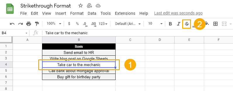
Below are the steps to add strikethrough format from the Toolbar.

1. Select the text you want to format with a strikethrough.
2. Click the Strikethrough icon in the toolbar. When you click on the strikethrough icon you will see it becomes green.

That’s it! Your selection will now have a strikethrough format!

This is a quick and easy method to add strikethrough formatting to any text.

If you want to remove strikethrough, select the cells where the formatting has already been applied and click on the strikethrough icon again, the formatting will be removed.

This is a great way to signify the data is no longer relevant without hiding the rows from view.

Add Strikethrough Format from the Format Menu

The second option for applying strikethrough is through the Format menu.

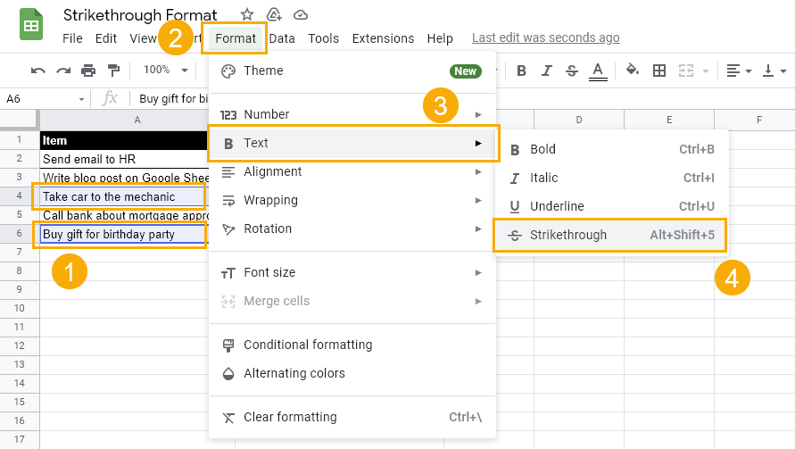
Follow these steps to add strikethrough from the format menu.

1. Select the cell where you want to strikethrough. This can be a single cell or a range of cells.
2. Go to the Format menu at the top of the page.
3. Select the Text option from the dropdown. It will open the submenu with all the text formatting options.
4. Select Strikethrough from the options.

Once you select strikethrough it is immediately applied to your selected text.

Add Strikethrough Format with a Keyboard Shortcut

You can also add strikethrough format with a keyboard shortcut if you prefer using your keyboard over the mouse.

To use this keyboard shortcut to strikethrough:

1. Select the cell where you want to apply the strikethrough formatting
2. Press Alt + Shift + 5 on the keyboard.

Hold the Alt and the Shift key together and then press the 5 key.

If you frequently use strikethrough formatting, the keyboard shortcut is the quickest way to speed up the process. It’s just a matter of remembering the keys. 😊

Add Strikethrough Format with Conditional Formatting

Strikethrough is commonly utilized when working with task lists or to-do lists.

What is a ToDo List? It’s a list of tasks you need to complete or want to do.

Here I have created a task list with the help of checkboxes and conditional formatting to automatically apply strikethrough.

Whenever you mark a checkbox, the text in the corresponding cell will get the strikethrough format applied.

This is a great visual indicator to signify the task has been marked as complete!

Conditional formatting plays a vital role in this solution and Google Sheets have made it straightforward to add strikethrough with conditional formatting.

All conditional formatting rules are based on simple logic, if a condition is true, then apply the selected format. In this scenario, formatting will be applied when you check any of the checkboxes.

The value in the cell checkbox cell is TRUE when the box is checked and FALSE when the box is unchecked. This value is then used in the conditional formatting rule to apply the strikethrough format.

Here’s how you can implement this conditional format scenario.

1. Select a range of cells where you want the checkbox. In this example all the checkboxes are in column A.
2. Click on Insert menu.
3. Choose Checkboxes from the options.

Cells with a checkbox either have a TRUE or FALSE value. If the checkbox is checked, the value is TRUE and if the checkbox is not checked, the value is FALSE.

You can see this by selecting any cell that has a checkbox and looking at the formula bar.

These Checkboxes are special checkmarks that allow you to toggle values.

The selection will have checkboxes added.

4. Select the cell you to which you wish to add strikethrough format when the checkbox is checked. This is column B in this example.
5. Click the Format menu.
6. Then select the Conditional Formatting option. This will open the conditional formatting pane on the right.

7. Click on the Add new rule option in the Conditional format rules pane.

8. Click on the Format cells if drop-down and select Custom formula is.
9. Enter =A2 in the Value or Formula box.
10. Select the Strikethrough format in the Formatting style section. You can also specify any additional formatting if you want.
11. Click on the Done button.

This will apply the strikethrough format to all the items where the Checkbox is ticked.

Conditional formatting is dynamic, so if you check any of the checkboxes the corresponding cell will automatically get the strikethrough format applied. Also, when you uncheck a box the strikethrough will be removed.

Add Strikethrough Format with an Apps Scripts

If you prefer, you can automate the process of adding strikethrough format with the help of App Scripts.

Go to the Extensions menu and select Apps Script to open the script editor.

Without adding any formatting manually, this script will automatically add strikethrough,

The only thing you need to do is check the check box and strikethrough will be inserted into the adjacent cell.

This is possible because of the onEdit trigger used in the Apps Script.

This lets you automatically run Apps Script functions when specific events occur. The onEdit trigger will run when a user changes a value in the spreadsheet.

Every time the spreadsheet notices a change in the cell, it checks if the checkbox value is set to True.

If the value is true, it changes the font line style to line-through for the adjacent cell using the SetFontLine class.

When the checkbox is unchecked and the value is set to false, and the script sets the font style as null.

function onEdit(e){
  var mySheet = SpreadsheetApp.getActiveSpreadsheet().getActiveSheet();
  var myRange = e.range;
  var mySheetName = mySheet.getSheetName();
  var myStatus = myRange.getValue();
  var currRow = myRange.getRow();
  var currCol = myRange.getColumn();
  var myItem = mySheet.getRange(currRow, currCol + 1);
  if (
    mySheetName === 'Apps Scripts'
    && currCol === 1
  ) {
    if (
      myStatus
    ) {
      myItem.setFontLine("line-through");
    } else {
      myItem.setFontLine(null);
    };
  };
};

You can write the script if you are familiar with the code in Apps Scripts, or else you can directly copy and paste the script code above into the Apps Script environment.

mySheetName === 'Apps Scripts'

The only change you will have to make is to update or change the Apps Scripts sheet name in the above line of code to whatever your sheet name is.

With this small script, you will be able to add strikethrough format to any Google Sheet you are working on.

Remove Strikethrough Format

You have so far seen various methods to apply strikethrough format. Now I’ll show you how to remove any strikethrough format.

Like other formats in Google Sheets, you can remove strikethrough by repeating the same process followed when adding the format.

The strikethrough commands all act as a toggle switch, so they will either add or remove the format depending on the current state.

This is applicable for the Toolbar, Format menu, and keyboard shortcut methods of applying strikethrough format.

Remove Strikethrough Format with the Toolbar

Just select the cells that have the strikethrough format and click on the strikethrough option of the toolbar.

Remove Strikethrough Format with the Toolbar

Select the cells that have the strikethrough format ➜ go to the Format menu ➜ select Text ➜ select Strikethrough from the options.

Remove Strikethrough Format with a Keyboard Shortcut

To use the keyboard shortcut:

1. Select the cells from which you want to remove the strikethrough format.
2. Press Alt + Shift + 5 on the keyboard.

Remove Strikethrough Format from Conditional Formating

Strikethrough added using conditional formatting cannot be removed using the previous methods. You will have to remove the conditional format rule.

To remove a condition formatting rule follow these steps.

1. Go to the Format menu.
2. Select the Conditional Formatting option. It will open the Conditional format rules pane, which shows a list of all the formatting rules.
3. Click on the Trash icon and it will remove the conditional formatting.

Remove Strikethrough Format from Conditional Formating

The strike though applied by the script can be easily removed using any of the first three methods, but you will need to remove the script in order to prevent any further strikethrough from being added.

1. Open Project Editor using Apps Script option in the Extensions menu.
2. Select Project you want to delete and click on vertical dots available on the pane.
3. Click Delete and it will delete the project.

Remove Strikethrough Format with Clear Formatting Command

You can also use the Clear formatting command to remove any strikethrough format as well. Follow these steps to use this option.

1. Select the cell you want to remove the strikethrough formatting from.
2. Click the Format menu.
3. Choose Clear formatting from the options.

This can be achieved through the keyboard shortcut Ctrl + \ as well.

But the only challenge you will face is by using this option is it removes all other formats on the selected cell.

Conclusions

Now you should have all the knowledge you need to properly add strikethrough in your Google Sheets.

You can also copy-paste strikethrough from one cell to another cell using the format painter.

Strikethrough can be applied to any type of data, such as text, number, date, or boolean.

Depending on what you need your data to do, you can use these easy techniques for adding strikethrough to your Google Sheets.

Have you used strikethrough in your Google Sheets? Do you have any other method to apply strikethrough? Which one is your favorite method?

Share your thoughts in the comment section below!