This post is going to show you all the ways you can add serial numbers to your data in Google Sheets.

What is an essential column in any database? Data Analysts will agree that the serial number, ID, row number, or key column is of utmost importance.

Regardless of the size of your dataset, you will usually need a serial number.

Adding a serial number can be a straightforward task. It is indeed when you know the various easy ways of doing so which can save you a significant amount of time over manually entering numbers.

Typing numbers manually is definitely one way to produce serial numbers, but when you have datasets with thousands of rows it won’t be possible to add them cell by cell.

Throughout this article, you will learn all the easy ways you can use to add serial numbers in Google Sheets. Get your copy of the example workbook to follow along!

Insert Serial Numbers with the Default Row Numbers

The first method to add serial numbers actually requires you to do nothing.

You heard it right! You don’t need to add anything to your Google Sheets. Each spreadsheet contains default row numbers that can work as serial numbers for you.

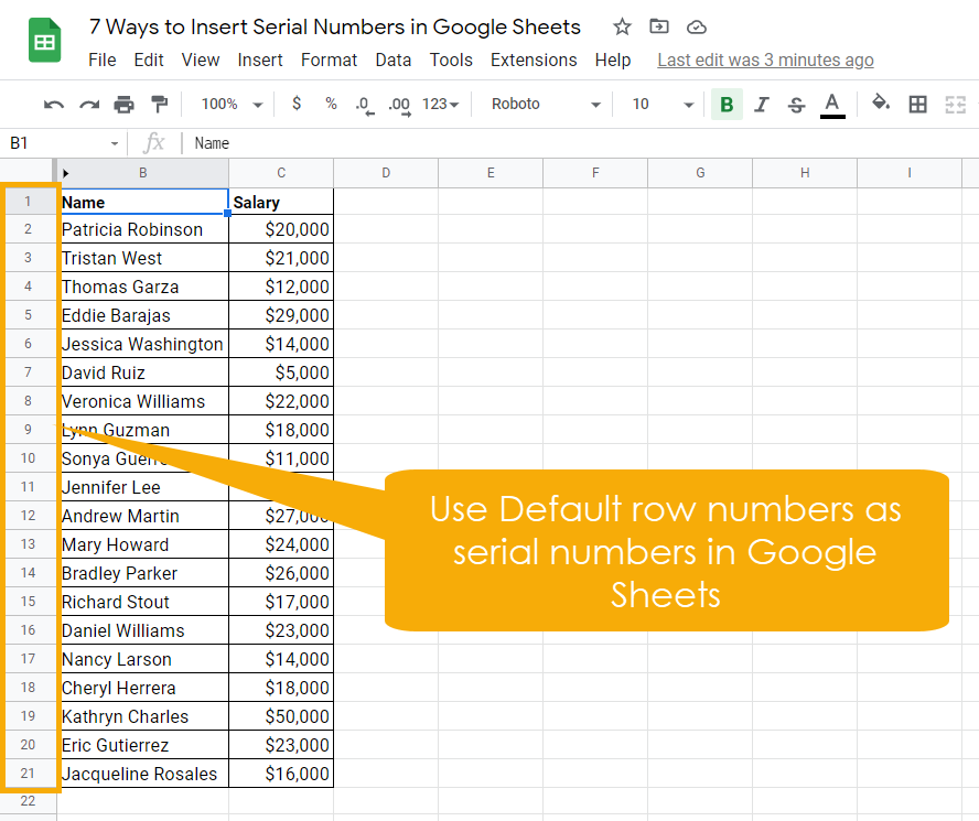
This method can sometimes be overlooked when using Google Sheets as an input database. But most of the tools you use are going to accept the default row numbering.

Insert Serial Numbers Using the Fill Handle

If you are using Google Sheets, this method will be a blessing for you. You will be able to add serial numbers with a few clicks for large datasets by using the Fill Handle to populate serial numbers.

The Fill Handle tool in Google Sheets allows you to autocomplete the list of serial numbers with your mouse.

Suppose you want to add serial numbers in column A for the database shown in the previous example. Using the Fill Handle, you can add those very quickly, without the need to type them manually.

There are three different ways you can use the Fill Handle. You will learn each through this section.

Fill Handle with Click and Drag

You can use the Fill handle and left mouse key to drag the cells down and fill the cells with a list of sequential numbers. This method is better for smaller datasets as it requires dragging down to the last row.

1. Type the first two serial number manually as shown in the screenshot above. A minimum of two cells are required to define the sequence required.
2. Select the cells containing those two serial numbers. You will see that a blue solid square box will appear on the bottom right hand side of the selection. That is the Fill Handle. It can automatically fill the remaining cells with a sequence of numbers increased with a step of 1 unit.

3. Keep the mouse cursor on that solid square of Fill Handle.
4. Hold the left mouse key and drag the cursor down to the end of your dataset to fill the cells with a sequence of numbers.

Congratulations! You have successfully added the serial numbers with Fill Handle.

Fill Handle and Double Click

Another way of using the Fill Handle is by double-clicking the solid square icon in the column.

This works exactly the same way the drag-down method works. Once you double-click on the Fill Handle icon, it will populate the list of sequential numbers.

How does it know at what cell to stop? The intelligence of Google Sheets checks for the last working row of the adjacent column and populates the sequence to the end of that row.

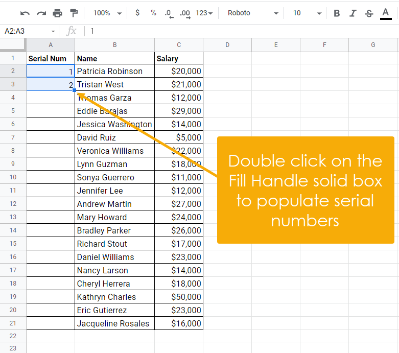
1. Add the first two serial numbers and select both cells.
2. Double click on the Fill Handle.

Google Sheets will populate the serial numbers down the rows until the last working row.

Fill Handle with the Ctrl Key

There is another exciting feature of the Fill Handle you might not know.

You can use it with the Ctrl key to drag the cells down. Google Sheets will identify that you want to create a sequence of numbers based on the first cell value.

You don’t need to type the first two numbers to identify the pattern. Adding a single number and then dragging is okay with this method.

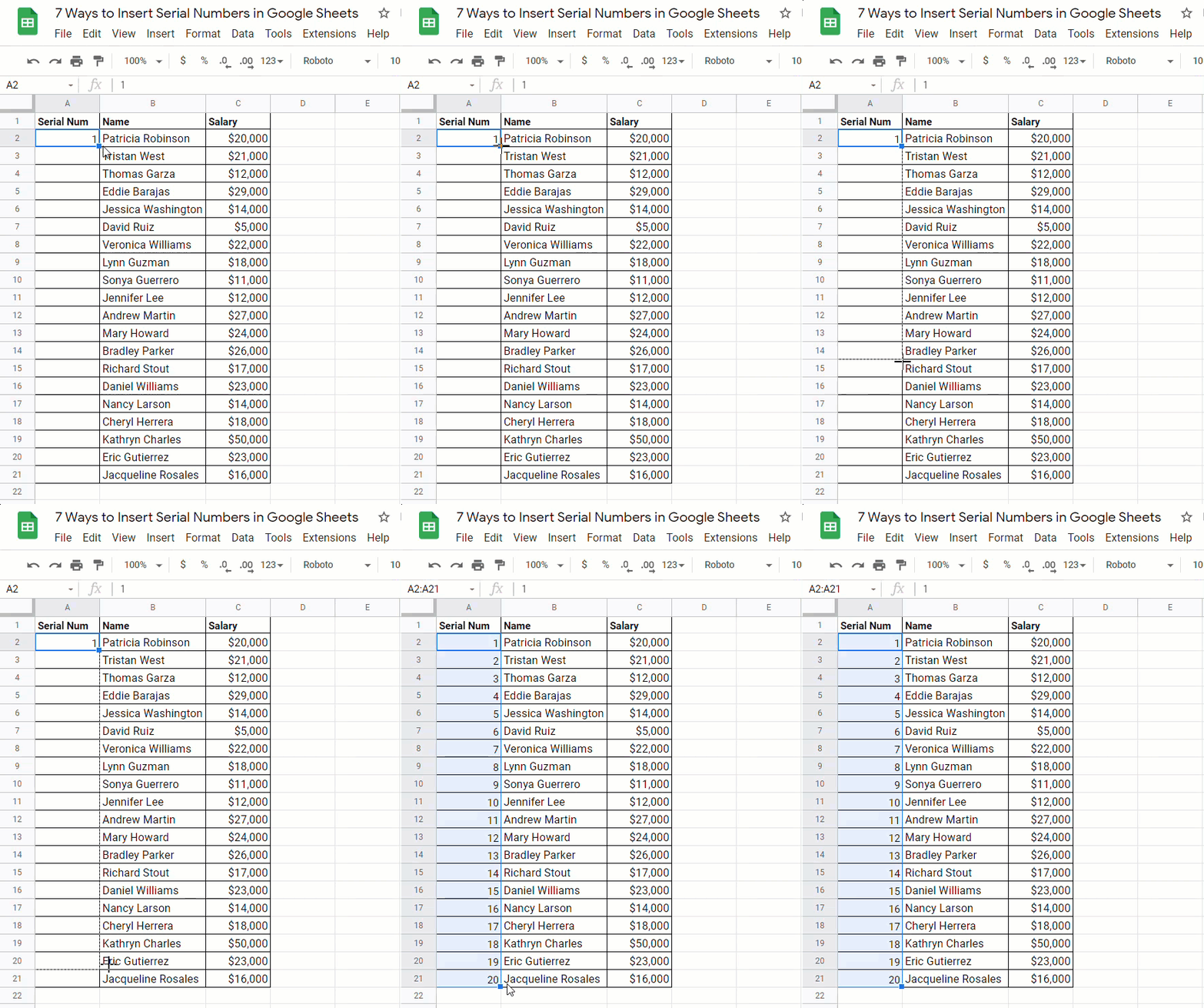
1. Type the first serial number in the cell.
2. Hold the Ctrl key on your keyboard and left click and drag the Fill Handle down across the cells to the last row.

Google Sheets will fill the series of numbers with an increment of 1 unit in each subsequent cell.

Pro Tip: You can also hold the Ctrl key and double-click on the Fill Handle square solid box to generate the serial numbers.

Insert Serial Numbers by Adding One to the Previous Number

Adding one to the previous number is a simple yet effective method to create a list of serial numbers inside Google Sheets.

The method is dynamic due to the use of formulas.

There are different ways you get this done. You can type the number 1 in the first cell and then in the next cell, use the + operator to add the previous cell value and copy the formula down the rows to generate serial numbers.

In this way, the formula is not uniform across the entire column as the solution requires a hard-coded value in the first cell. Though it is effective and less tedious, there are always better ways!

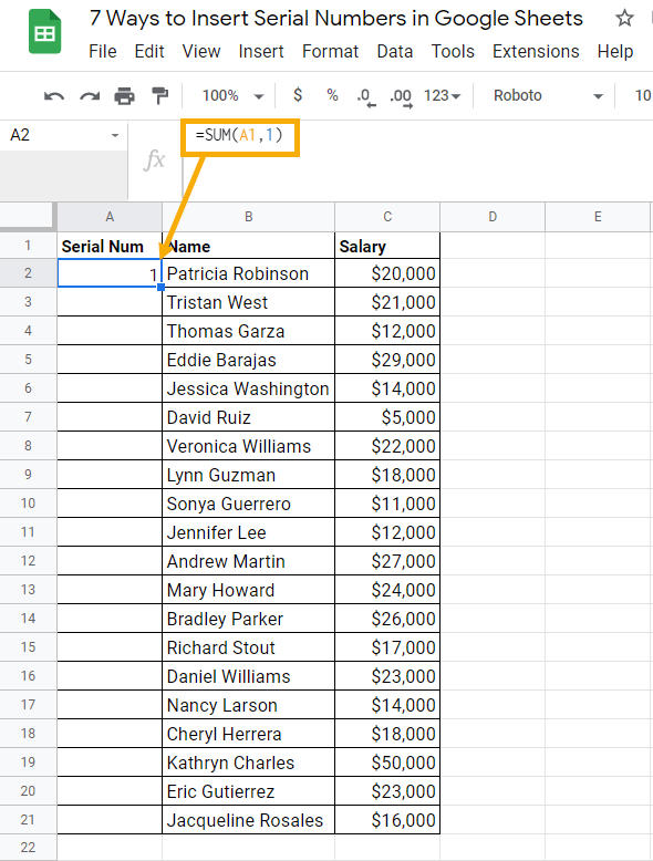
= SUM ( A1, 1 )

To add serial numbers by adding 1 to the previous number, type the above formula in cell A2 and hit the Enter button.

The function takes A1 as a value1 argument and 1 as a value2 argument. Since cell A1 contains a text column header, the formula will consider it as 0. Adding 0 with 1 will return 1 as the value in cell A2.

This solution avoids the hardcoded initial value with a uniform formula for the entire column while still achieving the desired sequence.

Now you can drag this formula down to the last row.

This way in A3, the formula will be =SUM(A2,1). Since A2 has value 1, the formula will return the number 2 in cell A3. Similarly, cell A4 will have number 3 and so on until the end.

Pro Tip: Instead of dragging the formula down, you can double-click on the Fill Handle to populate the formula down the rows.

Insert Serial Numbers with the ROW Function

Google Sheets has a lot of functions you can use to add serial numbers.

This method is a good option if you want to automatically update the serial numbers when you add or delete rows in the dataset.

The ROW function from Google Sheets any argument input and will return the row number of the current row. You can add a cell reference as an optional argument, and the ROW function will return the row number of that reference.

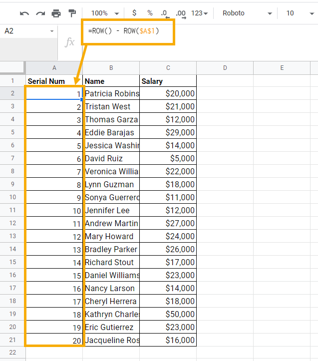
= ROW() - ROW ($A$1)

1. Add the above formula into cell A2.
2. Copy and paste the formula down the rows.

ROW() will return row number as 2 since the current cell is A2. ROW($A$1) will evaluate to 1 since it is referencing cell A1. This means the formula subtracts 1 from the current row number.

=ROW() - 1

Instead of subtracting ROW($A$1), you could hardcode this as 1 in the formula. But you would need to update the formula if you ever insert rows above the column headings in row 1.

Number Rows Using the COUNTA Function

The COUNTA function takes a range of cells and returns the count of non-empty cells. You can use this function to generate serial numbers.

If you are looking for a method that can return a serial number for only those rows that are filled with values or non-empty, then using this function is the best way.

The COUNTA function won’t count a blank cell, the serial number will not increment even if you drag the formula down until the last row of your sheet.

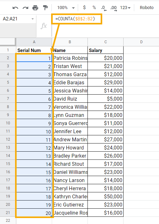
= COUNTA ( $B$2:B2 )

1. Add the formula =COUNTA($B$2:B2) to cell A2.
2. Drag the formula down the rows to the end of your data.

The first part of the range is fixed with the $ operator. The second part of the range is relative and it will change as the formula is copied down the rows.

This way, the formula counts the number of non-empty cells up to and including the current row.

= IF ( ISBLANK ( B2 ), "", COUNTA ( $B$2:B2 ) )

This can be combined with an IF function as above. This way no number is shown for rows with no data.

Insert Serial Numbers with the SEQUENCE Function

There is a function in Google Sheets that is specifically for creating sequences of numbers. This is the SEQUENCE function.

This function can generate an array of values from a single formula.

Syntax for the SEQUENCE Function

=SEQUENCE(rows, [columns], [start], [step])

• rows is a mandatory argument that specifies the number of rows to generate.
• columns specifies the number of columns to return. It is an optional argument, and if not specified it will defualt to 1.
• start is the number from which the sequence should start. It is an optional argument, and if not specified, the sequence will start from number 1.
• step is an optional argument that specifies the amount to increment the sequence. If not specified, the default step value is 1.

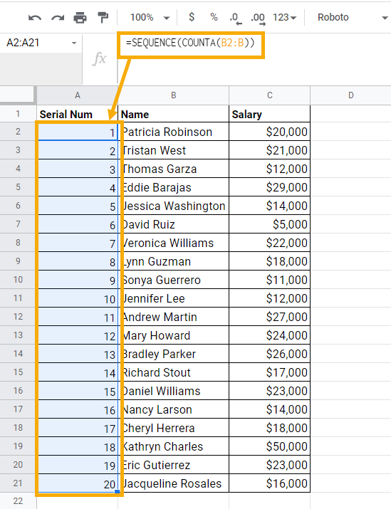
=SEQUENCE(COUNTA(B2:B))

In cell A2, insert the above formula to add an array of serial numbers.

The COUNTA function counts the number of non-empty rows from B2 onward. That number is then used as the row argument in the SEQUENCE function. In this example, a sequence of 20 numbers is generated across cell A2:A21.

As you add new rows with data in column B, the sequence will expand accordingly.

=SEQUENCE(20)

Another approach is to hardcode the row argument in the SEQUENCE function. The above formula creates a sequence from 1 to 20, but you would have to edit the row argument manually to add more rows.

Insert Serial Numbers with the ARRAYFORMULA Function

Another way to add row numbers in Google Sheets is using the ARRAYFORMULA in combination with the ROW and INDIRECT function.

The ARRAYFORMULA function allows you to use arrays with functions that don’t normally support them as an argument.

This is one of the many great functions available only in Google Sheets.

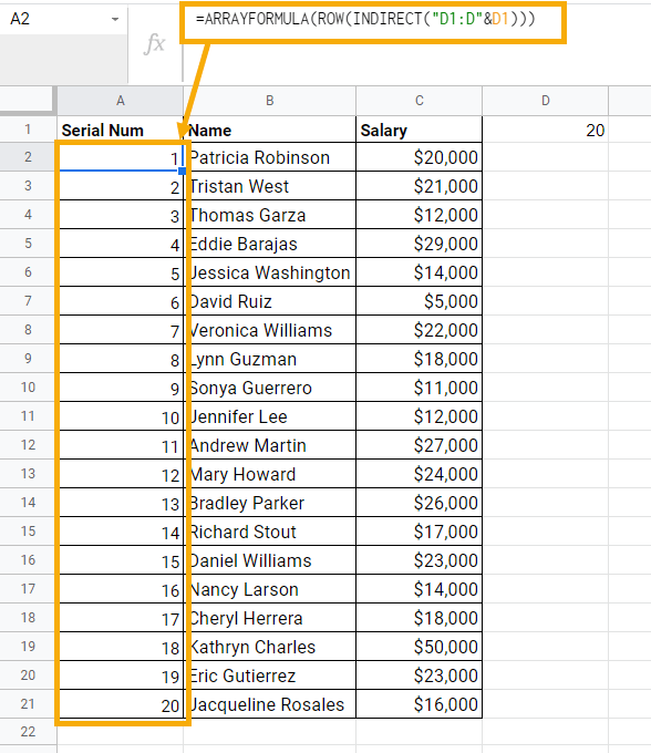
= ARRAYFORMULA ( ROW ( INDIRECT ( "D1:D" & D1 ) ) )

Insert the above formula in cell A2 to generate serial numbers. Cell D1 should contain the number of rows you want to add a sequence.

The INDIRECT function has the string value “D1:D” which is combined with the value in D1. In this case, it returns the cell reference D1:D20. This reference is then used as an input to the ROW function to generate the sequence of 20 numbers.

The ARRAYFORMULA function forces the output of an array instead of a single value.

= ARRAYFORMULA ( IF ( B2:B <> "", ROW ( A2:A ) - 1, "" ) )

You can also use the above formula to get the same result.

The IF function checks if column B is blank. ROW(A2:A)-1 will evaluate and return the row numbers if column B is not blank. Otherwise, it will return a blank value.

ARRAYFORMULA is used to return an array from these functions.

Number Rows Using the Apps Script

Apps Script is another way you can use to create serial numbers in Google Sheets.

Check out the full guide to apps scripts for more on Google Apps Scripts.

function addSequence() {
  var selectedRange = SpreadsheetApp.getActive().getSheetByName("Apps Script").getActiveRange()
  var selectedColumns = selectedRange.getWidth();
  var selectedRows = selectedRange.getHeight();
  var resultsArray = [];

  for (var i = 0; i < selectedRows; i++) {
    var rowData = [];
    for (var j = 0; j < selectedColumns; j++) {
      rowData.push(i * selectedColumns + j + 1);
    }
    resultsArray.push(rowData);
  }
  selectedRange.setValues(resultsArray);
}

Go to the Extensions menu and click on the Apps Script to open up the script editor. It will open up in a new browser tab. Copy and paste the code above below into the Apps Script.

Press the Save button in the upper ribbon then you can Run the script.

Explanation

• The first line of code defines the function named addSequence(). The function keyword defines it in the Apps Script. This is the function that will hold the entire piece of code that’s going to automate the process of adding the serial numbers.
• You need to specify the range that you selected in the sheet. The getActiveRange() method captures the active range and results are stored into the variable names as selectedRange.
• The height and width of the active range are returned by the getHeight() and getWidth() method and the results are stored into the selectedRows and selectedColumns respectively.
• A blank array that can hold the sequence results created from the loop is defined as resultsArray.
• A loop through each each cell in the active range is created and the sequence is added in the resultsArray during this look.
• The setValues() clause is used over selectedRange to push the data from resultsArray to the selected range A2:A21.

To run this script you will need to select the range in your sheet where you want to add the serial numbers.

In the Apps Script editor, press the Run button to execute this code and return the serial numbers inside your selected range. The code above will add a series of numbers starting from 1 and with step 1 across the selected range.

Conclusion

Throughout this article, you have learned many ways of adding serial numbers in Google Sheets.

Though the default row numbers can’t be customized, they can be handy sometimes.

The Fill Handle method is an easy way to create a static sequence with just a few mouse clicks.

But due to the static nature of the Fill Handle, it can’t automatically create serial numbers for any new rows that are added.

There are several formula methods available that can achieve serial numbers in a more dynamic fashion. The SUM, ROW, COUNTA, INDIRECT, and ARRAYFORMULA functions can all be used to return a sequence of row numbers if used correctly.

The SEQUENCE function is an easy formula alternative as it is dedicated to creating a numeric sequence of numbers down the rows and it is an excellent way to add your serial numbers in Google Sheets.

Do you have a favorite method to create row numbers? Let me know in the comments below!