Do you need to filter your data based on a strikethrough format? This post is going to show you how you can filter the strikethrough items of your list in Google Sheets.

Often times people will use the strikethrough format to indicate an item in their task list has been completed. While this can be a great visual indicator, it is a poor method for tracking since there are no tools available to filter based on this format.

Any further analysis based on the strikethrough format is nearly impossible! Fortunately, this tutorial will show how with two easy methods that will make filtering strikethrough a breeze.

Get your copy of the example workbook and follow along to learn how to filter your strikethrough data.

Custom App Script STRIKETHROUGH Function

Two methods will be discussed in this post, using a helper column, and using the FILTER function.

Both methods will depend on the use of a custom function.

Go to the Extensions menu and select the Apps Script option to open the code editor.

function STRIKETHROUGH(range) {
  //Get the formula from the current cell
  var currRange = SpreadsheetApp.getActiveRange();
  var currSheet = currRange.getSheet();
  var currFormula = currRange.getFormula();

  //Parse the function input parameter and convert it to a range reference
  var paramInput = currFormula.replace(/.*STRIKETHROUGH\(/gi, '').replace(/\).*/gi, '');
  var range = currSheet.getRange(paramInput);
  var styles = range.getTextStyles();
  var output = [];
  
  for (var i=0; i < styles.length ; i++) {
    var rows = [];
    for (var j=0; j < styles[0].length ; j++) {
      rows.push(styles[i][j].isStrikethrough());
    }
    output.push(rows)
  }
  return output
};

Copy and paste this script into your apps script editor window.

The script creates the custom function which you can call using the STRIKETHROUGH command. You can use this function after refreshing the spreadsheet.

= STRIKETHROUGH ( B2 )

The STRIKETHROUGH function checks if a cell has a strikethrough formatting and returns a true or false.

Filter Strikethrough Format with a Helper Column

Now that there’s a function that can check a cell for strikethrough formatting, the rest of the task becomes easier.

This method involves using a helper column to filter for strikethrough format.

= STRIKETHROUGH ( B2 )

Add a new Strikethrough column to your dataset with the above formula where B2 is referencing a column that will contain the strikethrough format.

After the custom function returns a true or false, you can then apply a filter to each column. You do this by selecting any cell in the range, going to the toolbar, and clicking on the filter icon.

📝 Note: If your screen is zoomed above 100%, click on the ellipse to reveal the remainder of the options where you will find the filter icon.

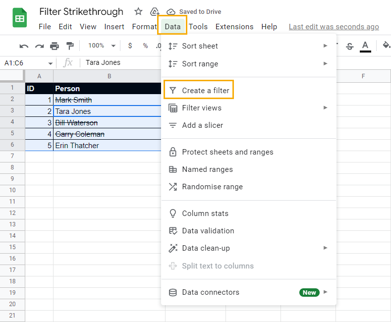
You can also apply the filter from the Data menu and select the Create a filter option.

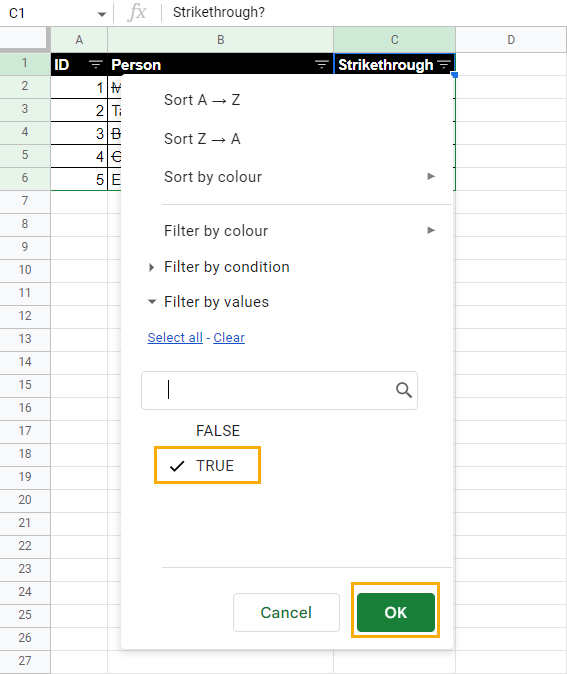
Click on the filter icon, then remove the FALSE cells in the Strikethrough column. Then select TRUE and click OK.

Now, all the cells left are those containing a strikethrough format.

💡 Tip: You can apply strikethrough format to your data automatically with conditional formatting. This way you will create a status column that can be used to filter your data in a more straightforward manner.

Filter Strikethrough Format with the FILTER Function

This method also involves filtering. However, it uses the FILTER function this time.

= FILTER ( range, condition1, [condition2, …] )

The FILTER function simply filters a range using specific conditions that evaluate to true or false.

= FILTER ( A2:B6, STRIKETHROUGH ( B2:B6 ) )

Using the above formula syntax will return the columns with data that have strikethrough formatting. The syntax filters the data using cells in B2:B6 that have strikethrough formatting.

The STRIKETHROUGH syntax returns true or false for each row.

Cell B2 for instance has a strikethrough formatting, so the condition reads true. As a result, the FILTER function returns the data in that row. This process continues for data in the other rows.

Conclusions

Using strikethrough format to indicate an item as complete is a common practice. But this makes viewing only the complete items a problem since there is no way to filter on strikethrough format.

It is possible to create a custom app script function that can show the strikethrough status of a cell. This will allow you to use two options for filtering cells with a strikethrough.

Using a helper column allows you to use the regular filter feature to show only the strikethrough items.

The custom function can also be used with the FILTER function to make the solution more dynamic as well as it allows you to filter strikethrough data in a different sheet.

Are there other methods for filtering strikethrough formatting that you know? Let me know down in the comments!