Do you want to learn how to fill down a formula in Google Sheets?

In this blog post, we’re going to show you all the different ways to do it. We’ll also explain the benefits of each method and when you might want to use them.

Google Sheets is a great productivity tool that provides various ways to work around the data you have. This includes creating new calculations with formulas.

One thing that you will do most often is to copy or fill a formula down the rows in Google Sheets. This is because of the tabular structure of your data where each column contains various rows, and you need to apply a formula to each row.

Copying the formula down across the rows or filling the formula down is a task you can do in seconds, provided that you know the proper technique.

By the end of this post, you’ll be able to fill down formulas with ease. So what are you waiting for? Get your copy of the example workbook and get started!

Fill Down a Formula with Copy and Paste

The crudest method of filling down the formula is copying and pasting it across the cells.

You don’t need to be a master of keyboard shortcuts or anything like that while working with this method. It’s just a simple copy and paste.

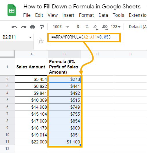
Suppose we have data as shown in the screenshot above, where column A consists of Sales Amount in USD.

In column B, you wish to apply a formula that captures the Profit, which is a simple 5% calculation of the Sales Amount.

In cell B2, type the formula =A2*0.05 or =A2*5%.

Both of these formulas produce the same result and generate 5% of the Sales Amount in cell B2.

Copy cell B2 using Ctrl + C. This will copy the formula in the cell.

Select the entire range from cell B3 to B11 and through your keyboard, hit Ctrl + V to paste it across the rows.

The formula will do its work and capture the 5% of revenue for each sales value present in column A.

Piece of Cake? It is indeed!

You can use this method to fill the formula down across the rows and generate the results.

Fill Down a Formula with Click and Drag

If you are working on a relatively smaller dataset such as a few hundred rows or less, then using the Click and Drag method is the best way to populate the formula down the rows.

This allows you to save time as you don’t need to copy and paste the values down across the rows.

While using this feature in Google Sheets, it recognizes the pattern across the rows. It then implements this over the remaining rows to generate a list with the same formulas.

To implement this method, click select cell B2 which contains the formula. Pay attention to the blue rectangle that appears as soon as you select the cell. This is the fill handle!

Hover your mouse cursor over the solid blue rectangle placed at the extreme right of the selected cell, and you will see the plus icon appearing with the fill handle.

Once you see the plus icon, click and hold on the left key of your mouse or touchpad and drag it down until cell B11.

Google Sheets identifies that you are trying to fill the cells with a formula and populates it across the cells.

You will see that the formula is filled down across the rows and captures the profit associated with each sales value.

Fill Down a Formula with Double Click

Another way that is faster than dragging the formula cell down across the cells is using the left mouse or touchpad key with a double click on the fill handle of the selected formula cell.

The method is more convenient as it allows you to copy the formula down even for a sheet with thousands of rows. You don’t need to worry about where the last row is for the formula.

Google Sheets is smart enough to check for the last working row and populate the formula until that point.

The formula is in cell B2 that captures the profit as 5% of the sales value from cell A2.

Select the cell and the fill handle will appear.

Hover your mouse over the fill handle and then double-click the left mouse key.

You will see that the formula is populated across the rows in column B for each row in column A until the last working row next to column A.

This utility saves you time as it automatically detects the last working row.

Fill Down a Formula with AutoFill

In 2020, Google Sheets added the AutoFill tool that allows you to either auto-complete a list or fills down a formula. This is by far one of the best features.

You can use this to complete a list by detecting patterns. It also automatically populates a formula down the rows and provides you with intelligent formula suggestions.

If you want to explore AutoFill more then you can read this post about all the ways you can use Smart Fill.

Type the formula =A2*0.05 in cell B2.

As soon as you hit the Enter button to execute the formula, the AutoFill window will pop up.

Click on the checkmark button to accept the suggestion. You can also use the keyboard shortcut Ctrl + Enter to AutoFill the formula down all the rows.

Fill Down a Formula with ARRAYFORMULA Function

There are a lot of very useful spreadsheet functions which you will only find in Google Sheets and ARRAYFORMULA should be at the top of this list because adds utility to many other functions.

Whenever you come up with a situation where a formula needs to be populated across the rows (as an array), the ARRAYFORMULA function is the way to achieve this.

ARRAYFORMULA allows you to convert formulae that result in a single cell value to an array of values.

= ARRAYFORMULA ( A2:A11 * 0.05 )

Select cell B2 and insert the above formula. This will output the calculation for each row in your data.

💡 Tip: There is a keyboard shortcut that will automatically wrap your formula with an ARRAYFORMULA function while in edit mode. Press Ctrl + Shift + Enter on the keyboard to convert the formula to an ARRAYFORMULA.

Fill Down a Formula with the QUERY Function

The QUERY function is very powerful due to its ability to work with arrays as SQL-Like databases.

It allows you to manipulate and transform data in almost any way imaginable. Moreover, it can return array values for row by row calculations.

If you wish to know more about this function, then check out this detailed guide to the QUERY function.

You can utilize the powerful QUERY function to fill a calculation down the rows in Google Sheets.

= QUERY ( A1:A11, "SELECT A*0.05" )

Insert the above QUERY function with the range A1:A11 as the data argument. There is no need to fix the range reference while working with the QUERY function since the single formula will return all the results.

Within the query argument, you can write a SELECT query. Since you want to capture 5% of column A, you must write the query argument as "SELECT A * 0.05" including the double quotations so it’s entered as text.

The formula performs a calculation for each row and returns the results in an array.

Apps Script to Automatically Fill Down a Formula

Apps Scripts allow you to write JavaScript code to automate your day-to-day activities in Google Sheets.

Interestingly, you can use the Apps Scripts to automatically fill the formula down across the rows in Google Sheets.

If you want to know more then check out this full guide to get started with Apps Scripts in Google Sheets.

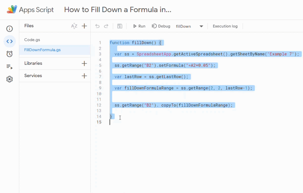
Go to the Extensions menu and select the Apps Script option to open the Apps Script editor in Google Sheets.

function fillDown() {
  var ss = SpreadsheetApp.getActiveSpreadsheet().getSheetByName("Example 7");
  ss.getRange("B2").setFormula("=A2*0.05");
  var lastRow = ss.getLastRow();
  var fillDownFormulaRange = ss.getRange(2, 2, lastRow-1);
  ss.getRange("B2"). copyTo(fillDownFormulaRange);
}

Copy and paste the above script code into the interface.

Explanation

This code will insert a formula into cell B2 and then copy it down to B11.

• fillDown() is the name given to this code using the function keyword. You can name it whatever you want, but having a descriptive name is always best.
• The SpreadsheetApp.getActiveSpreadsheet().getSheetByName() method allows you to access the sheet named Example 7. This is stored in a variable named ss.
• The getRange() method calls on ss and allows you to access cell B2. Then the setFormula() clause applies the formula =A2*0.05 in that cell.
• The getLastRow() method calls upon ss and gives you the last working row from your sheet. The results are stored in a variable named lastRow.
• The getRange() method is used to capture the range B2:B11 in a variable with the name fillDownFormulaRange.
• The copyTo() clause will then copy the formula stored in cell B2 down the range B2:B11.

Once you copy and paste the code, use the Run button from the ribbon inside Apps Script to run this script.

The Execution log will tell you the progress of this code running. Once it is completed, you will see the formula being populated across the rows in column B.

💡 Tip: You can use Apps Scripts to build your own custom functions such as this running total function that automatically fill down results.

Conclusions

There are many ways to fill down your formula calculations in Google Sheets.

A simple copy and paste is the easiest way and will get the job done.

Click and drag or double click methods can also be used to copy and paste formulas down the rows more quickly.

AutoFill can recognize the formula and last working row to populate the formula across those rows automatically. The method is versatile and quick. It also shows you the preview and allows you to either accept or reject the suggestions.

The ARRAYFORMULA function allows you to convert single value formulae into arrays to execute calculations on a row-by-row basis. You can reference all the rows at once on which the formula should be applied, and will automatically fill the results in each row.

The QUERY function is also helpful in filling down the calculation results across the rows by using an SQL query to achieve this result.

Finally, you can write a code of your own that works dynamically to fill the formula down the rows at a click of a button.

Which method do you use to fill down your formulas? Do you know any other tricks to achieve this? Let me know in the comments below!