In this post, you are going to see all the ways you can get a running total in Google Sheets.

The running total is the addition of a sequence of numbers such that every new number introduced to the sequence is added to the previous total. The running total is the cumulative addition of a series of numbers.

The running total concept has found use in various areas of business because it allows for easy identification of the total at any point in time.

For example, if you have a record of daily sales and you want to know the total sales year to date, you can easily find it with the running total.

Calculating the running total is a simple process, and Google Sheets has made it even easier.

In this post, you will learn the following 5 ways that you can use to get the running total.

• The addition + operator.
• The SUM function.
• The ARRAYFORMULA function.
• Custom Apps Script function.
• Pivot Table Calculated Field.

Get your copy of the example workbook with the above link to follow along!

Get a Running Total with the Addition Operator

This method doesn’t require you to use a function to get the running total. You only have to use the addition operator + to add up the cells you need.

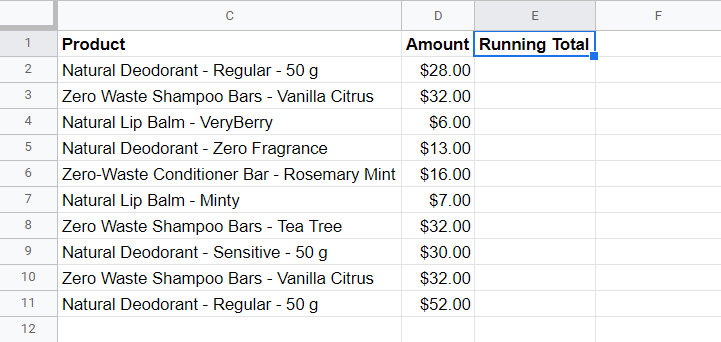
Follow these steps to get the running total for this sample data using the addition operator.

1. Enter =D2 into cell E2. This will copy the contents in cell D2 to cell E2.

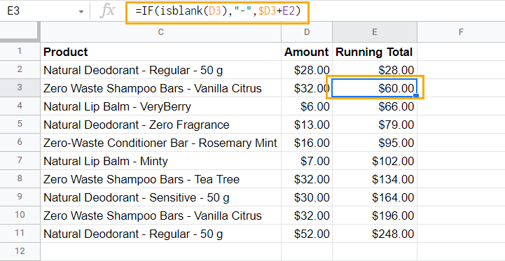
2. Enter the formula =D3+E2 into cell E3.

The formula will cumulate the total for the Natural Deodorant product and the amount of the Zero Waste Shampoo Bars product. This is the running total for the second row.

3. Drag down the fill handle to copy the formula to the empty cells.

When copying the formula into empty cells, you can run into a situation where you start to get a similar figure as the previous running total.

In this case, the figures in the Amount ends at row 11, but the formula has been copied further into row 15. Since the cells D12 to D15, the formula returns the same number.

In a large dataset where blank cells are present anywhere in-between, issues like that can be difficult to spot and correct.

You can wrap the formula in an IF function to prevent this problem.

= IF ( ISBLANK ( D3 ), "-", D3+E2 )

Copy and paste this formula in cell E3 and drag down the fill handle.

The IF function takes a logical expression and the values to return when the logical statement is true or false. In this syntax, the ISBLANK function is used to check if any cells in the Amount column are blank.

If the ISBLANK logical expression returns true, then the function will return a dash - character. If the logical expression is false, the function will return the running total operation.

The syntax allows you to format empty cells so that when you add new entries to the Amount column, the running total will automatically be calculated.

Get a Running Total with the SUM Function

In place of using the addition operator, you can use the SUM function to get the running total.

= SUM ( value1, [value2, …] )

The SUM function can add individual values or values from a cell range. It can take an arbitrary number of value arguments.

= SUM ( $D$2:D2 )

Copy the above formula into cell E2 to get the running total of the sample data and then copy and paste it down to the last row.

In the syntax, cell D2 has been fixed so that the summation range starts from cell D2 every time the formula is copied to a new row and new values are added.

= IF ( ISBLANK ( D2 ), "-", SUM ( $D$2:D2 ) )

You can troubleshoot the formula using the IF function like in the previous method to avoid showing a total when there is no data in the row.

Get a Running Total with the ARRAYFORMULA Function

More often than not, the first two methods will cover all your running total calculations needs.

The benefit of this method over the previous methods discussed is that you won’t have to copy down the formula.

This method will use a combination of the ARRAYFORMULA, SUMIF, and ROW functions.

= ARRAYFORMULA ( array_formula )

The ARRAYFORMULA function allows operations to return results in multiple rows and columns. It also allows the use of an array in functions that would normally not take an array. This attribute is crucial to our objective here.

Next up is the SUMIF function.

= SUMIF ( range, criterion, [sum_range] )

The SUMIF function returns the aggregate of a range based on a specific criteria.

= ROW ( [cell_reference] )

The ROW function returns the row number of a cell.

= ARRAYFORMULA ( SUMIF ( ROW ( D2:D11 ), "<=" & ROW ( D2:D11 ), D2:D11 ) )

To find the running totals copy and paste the above formula syntax into cell E2.

The benefit of using this method is that you don’t have to drag it down to copy the formula to other cells. You just enter the formula at the top of the column to calculate the running totals for all the rows.

Here’s a break down of how the formula works.

In the SUMIF function, the ROW in the range argument returns the row number for each of the cells in the range in an array. In this example, the ROW function returns {2, 3, 4, 5, 6, 7, 8, 9, 10, 11}.

The ROW function isn’t an array formula. But because it is inside an ARRAYFORMULA, it can take a range argument, and will also return the result in an array format. In this case, it returns the list of the row numbers in 11 rows.

The criterion argument of the SUMIF function doesn’t work with ranges. Because of this, the ROW function in the criterion argument behaves a little differently than the ROW function in the range argument.

The criterion argument doesn’t return an array, instead, it returns the row numbers of each cell in the range. The range is just used to specify which cell the operation should start and where to stop.

For instance, when the criterion argument calculates, the ROW function will return the number 2 for cell D2 and checks the range argument for rows that have numbers less than or equal to 2.

= ARRAYFORMULA ( SUMIF ( ROW ( D2:D11 ), "<=" & ROW ( D2 ), D2:D11 ) )

This is how the syntax will run when testing for cell D2.

After completing the operation for row D2, the syntax goes to the second cell in the range. In this case D3. For this, it will return 3 for cell D3.

= ARRAYFORMULA ( SUMIF ( ROW ( D2:D11 ), "<=" & ROW ( D3 ), D2:D11 ) )

This is how the syntax will run for cell D3.

When the criterion portion runs, it checks to find the cells in the range that meet the condition. Then the sum_range portion adds cells that meet the condition.

When the criterion argument is less than or equal to 2, the sum_range argument will add the value in cell D2 because only that cell in the range argument meets that condition.

When the criterion argument is less than equal to 3, then the sum_range argument will add up values in cells D3 and D2 because those are the cells that meet the criteria in the range argument.

The syntax continues to run this loop until it reaches the final cell in the operation.

Get a Running Total with a Custom Apps Script Function

Google spreadsheet provides a code editor that you can use to create custom functions. With an apps script, you can create functions that will automate repetitive tasks, and increase your efficiency.

To open the code editor window, go to the Extensions menu and click on Apps Script.

function RUNNINGTOTAL(myValues) {
  var selectedRows = myValues.length;
  var selectedColumns = myValues[0].length;
  var resultsArray = [];
  var runningTotal = 0;

  for (var i = 0; i < selectedRows; i++) {
    var rowData = [];
    for (var j = 0; j < selectedColumns; j++) {
      runningTotal = runningTotal + myValues[i][j];
      rowData.push(runningTotal);
    }
    resultsArray.push(rowData);
  }
  return resultsArray;
}

Copy and paste the above code syntax into the script editor.

Save the script and grant all the permission necessary to run the script in your spreadsheet. Then, go to your spreadsheet and refresh it.

You will now be able to use the RUNNINGTOTAL custom function in your spreadsheet.

= RUNNINGTOTAL ( D2:D11 )

The script creates a custom array formula called RUNNINGTOTAL. The function gets the values in the selected range and returns the running totals.

Unlike other methods, this custom function provides everything you need for calculating a running total in one place.

With RUNNINGTOTAL, you don’t have to combine two or more functions to get the running total.

= ARRAYFORMULA ( IF ( ISBLANK ( D2:D ), "-", RUNNINGTOTAL (D2:D) ) )

You can even go one step further with RUNNINGTOTAL by using the ARRAYFORMULA, IF, and ISBLANK functions to troubleshoot the formula.

With this syntax, you can format all of the cells in the Running Total column. The running total for every new entry is automatically calculated.

Get a Running Total with a Pivot Table Calculated Field

Pivot tables have features that help you filter, group, and sort fields that help you easily explore and identify various trends in your data.

What makes a pivot table different from regular tables is the kind of summaries you can generate.

Creating a pivot table in the spreadsheet is very easy. Follow these steps.

1. Select the range of data with which you want to work in the pivot table.
2. Go to the Insert menu and click on Pivot Table. The pivot table dialogue box that opens will pick up the already selected range.
3. Select the Existing sheet radio button to insert the pivot table into the existing sheet.
4. Select a cell and import the pivot table.

When the pivot table is inserted on the sheet, drag the Order Date field to the Rows section.

In the Values section, click on Add and select Calculated Field.

In the Calculated Field 1 box, under Summarise by, select Custom.

=SUMIFS($D:$D,$B:$B,"<="&'Order Date')

Delete the content inside the formula bar and paste the above formula syntax. The syntax uses the SUMIFS function to calculate the running total.

= SUMIFS ( sum_range, criteria_range1, criterion1, [criteria_range2, …], [criterion2, …] )

The SUMIFS function is similar to SUMIF. However, SUMIF takes only one criteria argument, whereas SUMIFS can return the sum of a range based on multiple criteria arguments.

The syntax used to arrive at the running totals adds the Amount column if the values in column B are less than and equal to individual Order Date values.

As the syntax goes through each Order Date value, it adds up all corresponding individual Amounts values that are less than or equal to a specific Order Date value.

For the syntax to work, the ranges have been locked in absolute references using the dollar sign, and the Order Date field needs to be sorted in ascending order.

You can change the default column header from Calculated field 1 by double-clicking on the cell.

Conclusions

You will most likely need to use only the addition operator or SUM function methods to calculate your running totals.

The other methods nevertheless will ensure that you cover any scenario where those two methods may not suffice.

Using an ARRAYFORMULA it is possible to return all the running total values from a single formula.

The custom apps script function might provide the best outlet for finding the running total. It’s a much better alternative as it will return all the running total calculations from a singe range input.

If you first need to summarize your data you can do this with a pivot table and calculate the running total inside the pivot table.

What other methods for finding the running totals do you know? Let us know in the comments section below!