This post is going to show you various ways you can use to display negative numbers in red inside your Google Sheets.

Formatting is a very powerful tool in your spreadsheet that allows you to easily spot and highlight important attributes of your data.

Displaying negative numbers with a red font color is a common technique that can help you easily see any values less than zero.

This is great for financial calculations to identify profit and loss, but you can also use these methods to format negative numbers with any color.

In this post, we are going to explore how you can use formatting to display negative numbers as red using these three methods.

• Custom number format.
• Conditional Formatting.
• Apps Script.

Get your copy of the example workbook to follow along.

Show Negative Numbers as Red with Custom Number Format

There are different number formats you can apply to your spreadsheet. A lot of the formatting options are already pre-set. With Custom number format, you can create your preferred formatting rules.

If you look closely at the sample data, there are a few negative numbers in the Profit column, but they are hard to spot with only the negative sign - to identify them.

You can apply a Custom number format to the Profit column so the negative numbers will become more easily visible.

You must first select the cells containing the numbers whose format you want to change before you start to apply the Custom number format.

Then follow these steps to access the Custom number format.

1. Go to the Format menu.
2. Select the Number option.
3. Click on Custom number format.

The Custom number format dialogue box will open.

The text box inside the Custom number format dialogue box is where you enter the Custom number format you want to apply.

In Custom number format, you can pass separate formatting instructions for four types of characters.

1. Positive: takes formatting instruction for positive numbers
2. Negative: takes formatting instruction for negative numbers
3. Zero: takes formatting instruction for displaying values
4. Text: takes formatting instruction for text characters

You pass custom formatting instruction using special symbols. For full details on these formatting symbols, follow this link.

When you’re done passing formatting instructions for one category, use a semicolon ; to signify the end of the formatting instruction for that category and the beginning of new formatting instructions for the next category.

#,##0;[Red](#,##0)
#,##0;[Red]#,##0
#,##0;-[red]#,##0

Copy and paste any of the above formats into the text box to display negative numbers as red.

The first syntax will display negative numbers in red with parenthesis. The second syntax will display negative numbers in red, but without parenthesis. The third syntax will display negative numbers in red, without parenthesis, but with the minus sign in front.

The display below the text box gives an instant preview of the formatting syntax on the numbers. After you’ve copied and pasted the syntax into the text box, click on the Apply button.

This will be your result when you use the first syntax.

This is the result when you use the second syntax.

This will be the result when you use the third syntax.

[green]#,##0;[Red](#,##0)

You can also take it a step further. Let’s say you want positive numbers to appear as green, just use the above syntax.

Show Negative Numbers as Red with Conditional Formatting

Conditional formatting is a pretty fantastic tool in Google Sheets. You can format cells based on specific conditions.

You will find Conditional formatting in the Format menu options.

After you click on Conditional formatting, a sidebar opens to the right of your spreadsheet. In the dialogue box, you can create and apply the rules with which you want to apply any formatting.

In Conditional formatting, formatting is applied to a cell or range of cells using color schemes. There are two options for applying cell colors in Conditional formatting. They are Single color and Color scale.

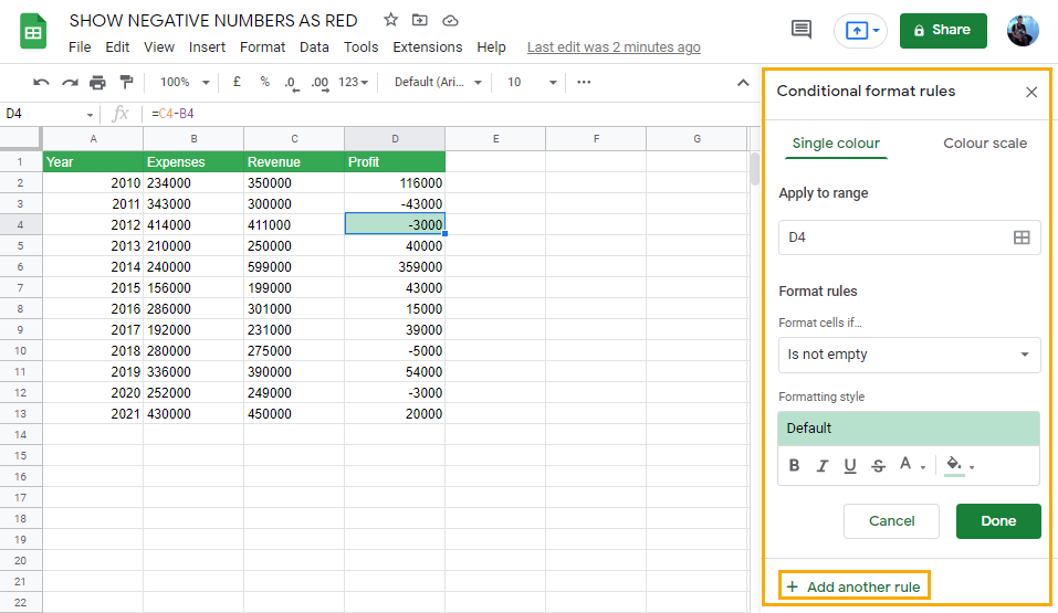
When the sidebar opens, the Single color option is selected by default, as seen in the above image. Under this category, you can only create one rule per range of cells and use one color per range of cells as well.

Using the Single color option, this is how to format negative numbers as red

Select the range of cells to which you want to apply the formatting. To do this, go to the Apply to range section and click on the small table icon to the right of the text box. If you place your mouse over the icon, you’ll see that it’s named Select data range.

This opens another dialogue box where you get a similar text box to input a range. In this dialogue box, you get an extra option to Add another range. This makes it convenient for you to apply the same formatting rules to multiple columns at the same time.

Select the cells or column that contains the data you want to apply Conditional formatting, then click on the OK button.

After you’ve selected the range of cells, you can then apply a format rule. Go to the Format rules section and select the drop-down arrow to reveal the Format rules options.

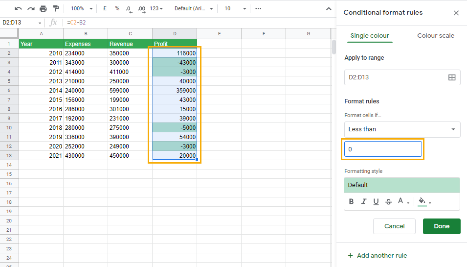
These are all the Format rules options for applying a conditional format. Because we want to format only negative numbers, we will use the Less than rule. You can experiment with the other options to understand how they work.

When you select the Less than rule, another text box appears underneath where you can insert the value against which the Less than rule is tested.

Any cells that are less than this value will be highlighted using a formatting style that you will specify in the next section.

Even without applying colors yet, you will see those cells less than zero in the Profit column have been highlighted in green. But we want to highlight them in red, so we will have to change the color.

After you’ve chosen a format rule, proceed to the Formatting style section to select which color to apply.

To apply red color to the cell, use the Fill color command.

Use the Text color command to apply font color formatting to the cell characters. You can apply other formatting options as you please.

When you’re done, click on the Done button to save the conditional formatting rule.

You can delete the rule with the delete icon. You can also use the Add another rule command to add more conditional formatting rules for the Single color section.

You can use the Colour scale formatting option to display negative numbers in red. As you will see, this option differs from the Single color option in various ways.

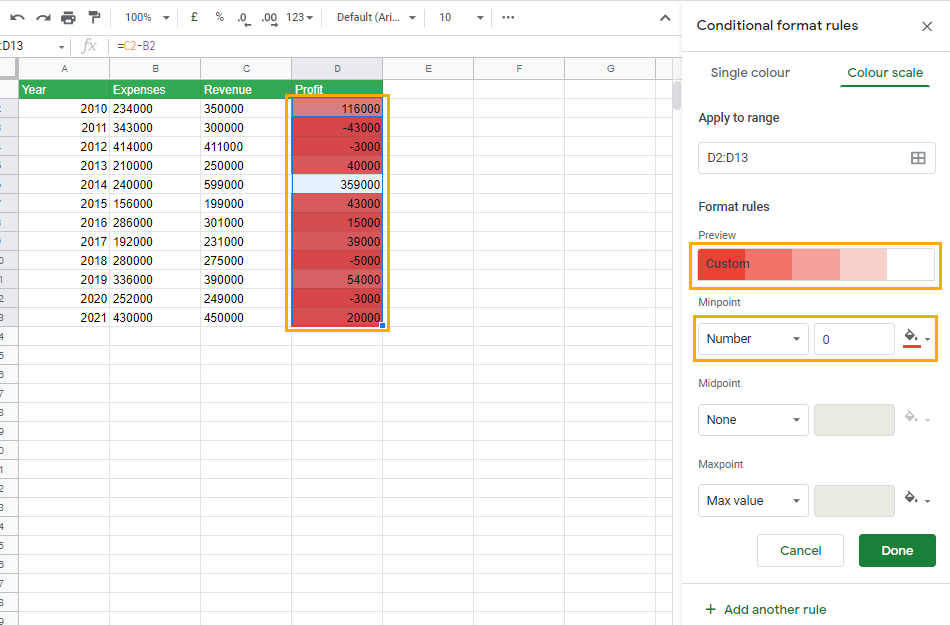
After selecting the cell ranges go to the Format rules section. You will see that there are three options for the rules you can apply. They are labeled as Minpoint, Midpoint, and Maxpoint.

Each category under the Format rules section has more specific rules that you can apply.

In the Minpoint category, you can set the minimum point using the Min value (minimum value) of the cell range you’ve selected.

Use the Number option to use a specific number as the minimum value. You can use the Percent and Percentile option to set portions of your selected range as the minimum value.

You also get the same options for the Midpoint and Maxpoint categories.

Beside each Format rules category is the fill color icon which you can use to specify colors for each rule.

In the Format rules section is a Preview of the color scales. It shows how the color scales will be applied in the cells from the minimum to the maximum value.

To format negative numbers as red using the Colour scale, select the Number option in the Minpoint Format rules category and set it to 0. Select the fill color command and choose the color red.

Because the color red has been applied, the Preview shows a color scale with the lowest values in dark red and the highest value in white. This is also reflected in the selected cell range.

To change the color of the other values, select the Number option in the Maxpoint section and set it to 0. Use the fill color to apply the color white.

Click the Done button to save the formatting or use the Add another rule command to add another rule.

Unlike the Single color option, the Colour scale option doesn’t allow you to apply font formatting to the cell. You can only apply a fill color to the cell.

Show Negative Numbers as Red with an Apps Script

You can also use a script to format negative numbers with a red font.

Go to the Extensions menu and select Apps Script from the options to open the script editor.

Check out this guide to Apps Scripts for details on how to use this great tool.

function changeNegColor() {
  var selectedRange = SpreadsheetApp.getActive().getActiveRange();
  var selectedValues = selectedRange.getValues();
  var selectedColumns = selectedRange.getWidth();
  var selectedRows = selectedRange.getHeight();

  for (i = 0; i < selectedRows; i++) {
    for (j = 0; j < selectedColumns; j++) {
      if (selectedValues[i][j] < 0) {
        selectedRange.getCell(i + 1, j + 1).setFontColor('red');
      } else {
        selectedRange.getCell(i + 1, j + 1).setFontColor('black');
      }
    };
  };
};

function onOpen() {
  var ui = SpreadsheetApp.getUi();
  ui.createMenu('Negatives')
    .addItem('Change Negative to Red', 'changeNegColor')
    .addToUi();
};

Copy and paste the above script into your script editor.

After pasting the script into the editor, make sure you Save and Run it before going back to refresh your spreadsheet.

The way the script works is simple. It uses the ui.createMenu method to create a custom menu called Negatives. After you refresh your spreadsheet, the custom menu will appear because of the onOpen trigger in the script.

To use the script to display the negative numbers in red, first select the range of cells you want to format. Go to the Negatives menu, then click on Change Negative to Red.

The script will loop through each value in the selected range and change the font color to red if the value is less than zero.

📝 Note: This method is not dynamic. If you change any values the font color will not update, but you can reuse the script to update the colors.

Conclusions

This article has shown you important ways you can use to format negative numbers to make them easily visible.

Without formatting the negative numbers will blend into the dataset, making it hard to spot them.

Custom number format, conditional formatting, and apps script methods can all be used to create negative numbers formatted in red.

Do you use any other formatting tricks to show your negative numbers in red? Let me know in the comments section below!